const: context data, and an axis that must not be cut

A sensor does not measure a spectrum, it measures a handful of bands, each one an average of the spectrum weighted by that band’s response:

\[L_b = \frac{\int R(\lambda)\, S_b(\lambda)\, d\lambda} {\int S_b(\lambda)\, d\lambda}\]

\(S_b\) is not being swept and is not produced by the call: it is context the engine needs, the same for every point. That is what const is for.

It also changes what may be done to the wavelength axis. The integral runs over all of it, so handing the engine one batch at a time would average each batch separately and quietly return the wrong number. The contract refuses that combination when the function is defined, not after the run.

Run with:

pixi run -e dev python examples/06_const_and_band_integration.py

from __future__ import annotations

import sys
from pathlib import Path

import matplotlib.pyplot as plt
import numpy as np
import xarray as xr

import xsweep

# sphinx-gallery executes examples without `__file__` set, so the gallery
# directory is located from the already-installed xsweep package instead.
sys.path.insert(0, str(Path(xsweep.__file__).resolve().parents[2] / "examples"))

from _solvers import (  # noqa: E402
    aerosol_optical_depth,
    rayleigh_optical_depth,
    spectral_doubling,
)
from xsweep import sweep  # noqa: E402
from xsweep.errors import ContractError  # noqa: E402

SSA = 0.95
ASYMMETRY = 0.65
WL = np.linspace(0.40, 2.40, 400)

# Synthetic Gaussian bands, loosely spaced like a land-imaging sensor's.
# They are not any real instrument's response functions.
BAND_CENTRES = np.array([0.49, 0.56, 0.665, 0.842, 1.61, 2.19])
BAND_WIDTHS = np.array([0.065, 0.035, 0.030, 0.115, 0.090, 0.180])

Building the response functions

Each row is normalised by its own sum, so the weighted sum below is an average rather than an integral that would need dividing afterwards.

srf = np.exp(
    -0.5 * ((WL[None, :] - BAND_CENTRES[:, None]) / (BAND_WIDTHS[:, None] / 2.355)) ** 2
)
srf /= srf.sum(axis=1, keepdims=True)

print(f"srf shape:      {srf.shape}  (band, wl)")
print(f"row sums:       {np.unique(np.round(srf.sum(axis=1), 12))}")

srf shape:      (6, 400)  (band, wl)
row sums:       [1.]

The contract

const(srf) hands the whole table to every call. It is not a sweep axis: the result has no srf dim, and the plan lists it among the arguments with its full shape.

CALLS = {"n": 0}


@sweep("loop(aot, pressure) vec(wl) const(srf) -> radiance(band)")
def bands(
    aot: float, pressure: float, wl: xr.DataArray, srf: xr.DataArray
) -> xr.DataArray:
    """Band-averaged reflectance for one atmosphere."""
    CALLS["n"] += 1
    tau = rayleigh_optical_depth(wl, pressure) + aerosol_optical_depth(wl, aot)
    reflectance = xr.DataArray(
        spectral_doubling(tau, SSA, ASYMMETRY)["reflectance"], dims="wl"
    )
    return (reflectance * srf).sum("wl")

The const variable lives in the space

It is an ordinary data variable of the Dataset, alongside the swept ones. What separates them is the contract, not the container.

space = xr.Dataset(
    {
        "aot": ("aot", np.array([0.05, 0.1, 0.2, 0.4, 0.8])),
        "pressure": ("pressure", np.array([700.0, 850.0, 1013.25])),
        "wl": ("wl", WL),
        "srf": (("band", "wl"), srf),
    },
    coords={"band": BAND_CENTRES},
)

print(bands.explain(space))

+- bands (v0) ------------------------------------------------+
| loop(aot, pressure) vec(wl) const(srf) -> radiance(band)
+------------------------------------------------------------+

SPACE
  aot        axis                 5
  pressure   axis                 3
  points                         15
  dedup                      disabled

CALLS
  to compute       15
  cached            0
  skipped           0
  total            15

ARGUMENTS
  aot          loop    float64
  pressure     loop    float64
  wl           vec     float64   [400]
  srf          const   float64   [6, 400]

RESULT
  radiance (aot: 5, pressure: 3, band: 6) float64

STORE      none (in-memory: no cache, no resume)
EXECUTOR   serial

result = bands(space)
print(f"{CALLS['n']} calls")
print(result)

15 calls
<xarray.Dataset> Size: 847B
Dimensions:   (aot: 5, pressure: 3, band: 6)
Coordinates:
  * aot       (aot) float64 40B 0.05 0.1 0.2 0.4 0.8
  * pressure  (pressure) float64 24B 700.0 850.0 1.013e+03
  * band      (band) float64 48B 0.49 0.56 0.665 0.842 1.61 2.19
Data variables:
    radiance  (aot, pressure, band) float64 720B 0.0524 0.0354 ... 0.061 0.04192
    status    (aot, pressure) uint8 15B 1 1 1 1 1 1 1 1 1 1 1 1 1 1 1
Attributes:
    xsweep_meta:  {'fingerprint': '354071029a64812f43e7a3cc878099da', 'contra...

The refusal

Ask for a batched wavelength axis alongside a const that reduces over it and the contract says no, at decoration time, before any engine has been started. The rule it applies is mechanical: a @ N marker only makes sense on an axis the output still carries, and radiance(band) has lost wl.

try:

    @sweep("loop(aot, pressure) vec(wl @ 100) const(srf) -> radiance(band)")
    def batched_bands(
        aot: float, pressure: float, wl: xr.DataArray, srf: xr.DataArray
    ) -> xr.DataArray:
        """This never gets defined."""
        raise AssertionError("unreachable")

except ContractError as error:
    print(f"ContractError: {error}")

ContractError: '@ 100' on 'wl', which is not among the declared output dims ['band']. Either the function reduces over that axis, and batching it would corrupt the result, so drop the marker to pass the whole axis in one call; or 'wl' is multi-dim, and batch sizes must then be declared per dim in the policy, e.g. chunks={"x": 500, "y": 500}

Compare that with page 05, where the output was reflectance(wl): the axis survived the call, so batching it was safe and was allowed. The contract is not guessing about the physics, it is reading what you declared the call produces.

The result

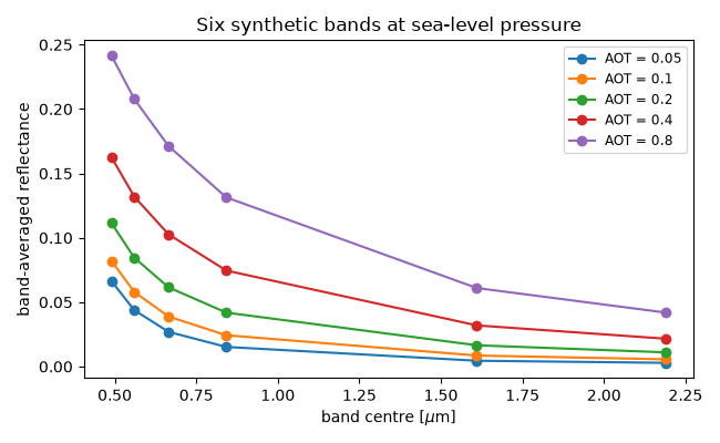
Six numbers per atmosphere instead of four hundred, and the aerosol signal concentrated where it can actually be told apart from molecular scattering.

fig, ax = plt.subplots(figsize=(6.5, 4.0))
for aot in space.aot.values:
    ax.plot(
        BAND_CENTRES,
        result.radiance.sel(aot=aot, pressure=1013.25),
        marker="o",
        label=f"AOT = {aot:g}",
    )
ax.set_xlabel(r"band centre [$\mu$m]")
ax.set_ylabel("band-averaged reflectance")
ax.set_title("Six synthetic bands at sea-level pressure")
ax.legend(fontsize="small")
fig.tight_layout()
plt.show()