vec: hand over the axis the engine already knows how to do

A function is rarely all-or-nothing about vectorisation. The doubling solver in this gallery is a sequential recursion in optical thickness, so a configuration goes in one at a time, but every operation inside it is elementwise, so a 400-point spectrum costs what one wavelength costs. Real spectral engines have the same shape: one atmosphere in, a spectrum out.

vec is how the contract says that. loop variables arrive one value per call; a vec variable arrives as a whole axis:

\[\tau(\lambda) = \tau_R(\lambda, p) + \tau_a(\lambda, \text{AOT})\]

with \(\tau_R\) from Bodhaine et al. (1999) and \(\tau_a\) the Angstrom power law. Pressure and aerosol loading are swept; wavelength is handed over whole.

Run with:

pixi run -e dev python examples/05_vec_a_whole_spectrum.py

from __future__ import annotations

import sys
import time
from pathlib import Path

import matplotlib.pyplot as plt
import numpy as np
import xarray as xr

import xsweep

# sphinx-gallery executes examples without `__file__` set, so the gallery
# directory is located from the already-installed xsweep package instead.
sys.path.insert(0, str(Path(xsweep.__file__).resolve().parents[2] / "examples"))

from _solvers import (  # noqa: E402
    aerosol_optical_depth,
    rayleigh_optical_depth,
    spectral_doubling,
)
from xsweep import SweepPolicy, sweep  # noqa: E402

SSA = 0.95
ASYMMETRY = 0.65
WL = np.linspace(0.40, 2.40, 400)

The engine is elementwise in wavelength

Sixteen doublings of a 400-point spectrum cost barely more than sixteen doublings of one number. Calling it once per wavelength would be pure waste, and it is exactly the waste a loop variable would create.

for n_wl in (1, 40, 400):
    tau = rayleigh_optical_depth(WL[:n_wl]) + aerosol_optical_depth(WL[:n_wl], 0.3)
    start = time.perf_counter()
    for _ in range(50):
        spectral_doubling(tau, SSA, ASYMMETRY)
    print(f"{n_wl:>4} wavelengths: {(time.perf_counter() - start) / 50 * 1e6:6.0f} us")

  1 wavelengths:     46 us
 40 wavelengths:     46 us
400 wavelengths:     61 us

The contract

aot and pressure are loop: one float per call. wl is vec: the whole axis, as an xr.DataArray. The outputs are declared with the dim they carry, reflectance(wl).

CALLS = {"n": 0}


@sweep("loop(aot, pressure) vec(wl) -> reflectance(wl), transmittance(wl)")
def spectrum(aot: float, pressure: float, wl: xr.DataArray) -> dict[str, xr.DataArray]:
    """Spectral reflectance of one atmosphere, by two-stream doubling."""
    CALLS["n"] += 1
    tau = rayleigh_optical_depth(wl, pressure) + aerosol_optical_depth(wl, aot)
    out = spectral_doubling(tau, SSA, ASYMMETRY)
    return {k: xr.DataArray(v, dims="wl") for k, v in out.items()}


space = xr.Dataset(
    {
        "aot": ("aot", np.array([0.05, 0.1, 0.2, 0.4, 0.8])),
        "pressure": ("pressure", np.array([700.0, 850.0, 1013.25])),
        "wl": ("wl", WL),
    }
)

Fifteen calls, not six thousand

The plan makes the distinction visible: wl is not an axis of the sweep, it is the shape of one call’s argument, so it appears under ARGUMENTS with its length rather than under SPACE.

print(spectrum.explain(space))

+- spectrum (v0) ---------------------------------------------+
| loop(aot, pressure) vec(wl) -> reflectance(wl), transmittance(wl)
+------------------------------------------------------------+

SPACE
  aot        axis                 5
  pressure   axis                 3
  points                         15
  dedup                      disabled

CALLS
  to compute       15
  cached            0
  skipped           0
  total            15

ARGUMENTS
  aot          loop    float64
  pressure     loop    float64
  wl           vec     float64   [400]

RESULT
  reflectance (aot: 5, pressure: 3, wl: 400) float64
  transmittance (aot: 5, pressure: 3, wl: 400) float64

STORE      none (in-memory: no cache, no resume)
EXECUTOR   serial

start = time.perf_counter()
result = spectrum(space)
print(f"{CALLS['n']} calls in {time.perf_counter() - start:.3f} s")
print(result)

15 calls in 0.023 s
<xarray.Dataset> Size: 99kB
Dimensions:        (aot: 5, pressure: 3, wl: 400)
Coordinates:
  * aot            (aot) float64 40B 0.05 0.1 0.2 0.4 0.8
  * pressure       (pressure) float64 24B 700.0 850.0 1.013e+03
  * wl             (wl) float64 3kB 0.4 0.405 0.41 0.415 ... 2.39 2.395 2.4
Data variables:
    reflectance    (aot, pressure, wl) float64 48kB 0.09439 0.09088 ... 0.03735
    status         (aot, pressure) uint8 15B 1 1 1 1 1 1 1 1 1 1 1 1 1 1 1
    transmittance  (aot, pressure, wl) float64 48kB 0.8737 0.8785 ... 0.9509
Attributes:
    xsweep_meta:  {'fingerprint': 'e2cdad267e6c9ce5b83988215f89a579', 'contra...

Batching the axis, without moving a value

A vec axis can be handed over in pieces when it is too large to hold at once: chunks keyed by dim, or the @ N marker in the contract. That is a memory decision, and it must not be a numerical one.

It is only safe because the engine is elementwise along that axis. The doubling depth is a fixed number rather than one derived from the data, so a slice cannot see a different recursion than the whole axis does. A function that reduces over the axis, or that needs its neighbours, is not safe to batch, and the contract refuses that case outright on the next page.

CALLS["n"] = 0
batched = spectrum(space, policy=SweepPolicy(chunks={"wl": 100}))
print(f"{CALLS['n']} calls with wl in batches of 100")

np.testing.assert_array_equal(result.reflectance.values, batched.reflectance.values)
np.testing.assert_array_equal(result.transmittance.values, batched.transmittance.values)
print("identical to the unbatched run, to the last bit")

60 calls with wl in batches of 100
identical to the unbatched run, to the last bit

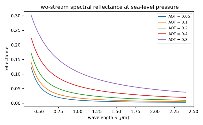
What the spectra look like

Rayleigh scattering falls off steeply with wavelength, so the blue end is where the atmosphere is bright and where aerosol loading is hardest to separate from the molecular signal.

fig, ax = plt.subplots(figsize=(6.5, 4.0))
for aot in space.aot.values:
    ax.plot(
        result.wl,
        result.reflectance.sel(aot=aot, pressure=1013.25),
        label=f"AOT = {aot:g}",
    )
ax.set_xlabel(r"wavelength $\lambda$ [$\mu$m]")
ax.set_ylabel("reflectance")
ax.set_title("Two-stream spectral reflectance at sea-level pressure")
ax.legend(fontsize="small")
fig.tight_layout()
plt.show()