Start here: an engine you cannot vectorise

If your function is a closed form, numpy already sweeps it: evaluate it over the whole grid at once and you are done. xsweep would add nothing.

This gallery’s engine is not that. mc_reflectance traces photons through a scattering layer one at a time, and each photon is a loop that ends when the photon leaves, after a number of collisions nobody knows in advance:

\[s = -\ln u, \qquad z \mathrel{+}= s\,\mu, \qquad w \mathrel{*}= \omega, \qquad \mu' = \mu\cos\Theta + \sqrt{1-\mu^2}\,\sqrt{1-\cos^2\Theta}\,\cos\varphi\]

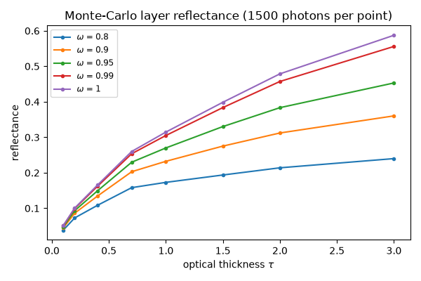
There is no array shape to broadcast over. The only way to cover a grid of optical thicknesses \(\tau\) and single-scattering albedos \(\omega\) is to call the thing once per point, which is what this page does twice: by hand, then with xsweep.

Run with:

pixi run -e dev python examples/01_why_a_sweep_library.py

from __future__ import annotations

import sys
import time
from pathlib import Path

import matplotlib.pyplot as plt
import numpy as np
import xarray as xr

import xsweep

# sphinx-gallery executes examples without `__file__` set, so the gallery
# directory is located from the already-installed xsweep package instead.
sys.path.insert(0, str(Path(xsweep.__file__).resolve().parents[2] / "examples"))

from _solvers import mc_reflectance  # noqa: E402
from xsweep import sweep  # noqa: E402

N_PHOTONS = 1500
TAU = np.array([0.1, 0.2, 0.4, 0.7, 1.0, 1.5, 2.0, 3.0])
SSA = np.array([0.8, 0.9, 0.95, 0.99, 1.0])

What one call costs

Everything downstream follows from this number. A gallery has to build a website, so n_photons is small here; a production run means seconds to minutes per point, and that is the regime the rest of this gallery is about.

start = time.perf_counter()
one = mc_reflectance(1.0, 0.95, g=0.6, mu0=0.5, n_photons=N_PHOTONS, seed=0)
per_call = time.perf_counter() - start

print(f"reflectance = {one['reflectance']:.4f}")
print(f"cost        = {per_call * 1e3:.1f} ms for {N_PHOTONS} photons")
print(f"grid        = {TAU.size} x {SSA.size} = {TAU.size * SSA.size} points")

reflectance = 0.2700
cost        = 6.5 ms for 1500 photons
grid        = 8 x 5 = 40 points

By hand

This is the loop everyone writes first. It works. It is also the reason this library exists: what comes back is a bare array whose axes live only in your head, with no record of what was computed and nothing left behind if the process dies at point 30 of 40.

start = time.perf_counter()
by_hand = np.empty((TAU.size, SSA.size))
for i, tau in enumerate(TAU):
    for j, ssa in enumerate(SSA):
        out = mc_reflectance(
            float(tau), float(ssa), g=0.6, mu0=0.5, n_photons=N_PHOTONS, seed=0
        )
        by_hand[i, j] = out["reflectance"]

print(f"{by_hand.shape} array in {time.perf_counter() - start:.2f} s")

(8, 5) array in 0.26 s

The contract: what one call consumes and produces

loop means one value per call, handed over as a plain Python float. The arrow names the outputs, and a multi-output callee returns a dict keyed by those names. The contract says nothing about how many points there are.

CALLS = {"n": 0}


@sweep("loop(tau, ssa) -> reflectance(), transmittance()")
def layer(tau: float, ssa: float) -> dict[str, float]:
    """Reflectance and transmittance of a scattering layer, by Monte-Carlo."""
    CALLS["n"] += 1
    return mc_reflectance(tau, ssa, g=0.6, mu0=0.5, n_photons=N_PHOTONS, seed=0)

The space is an ordinary Dataset

tau and ssa sit on distinct dims, so they multiply: 8 x 5 = 40 points. Nothing in the contract said that; the dims did.

space = xr.Dataset({"tau": ("tau", TAU), "ssa": ("ssa", SSA)})

What it will cost, before paying for it

explain resolves the whole sweep and stops without calling the engine once. Combined with the cost of a single call measured above, this is the answer to “how long will this take”, available before committing to it.

plan = layer.explain(space)
print(plan)
print(f"\nestimate: {plan.n_to_compute} calls x {per_call * 1e3:.0f} ms")
print(f"       ~= {plan.n_to_compute * per_call:.1f} s")

+- layer (v0) ------------------------------------------------+
| loop(tau, ssa) -> reflectance(), transmittance()
+------------------------------------------------------------+

SPACE
  tau        axis                 8
  ssa        axis                 5
  points                         40
  dedup                      disabled

CALLS
  to compute       40
  cached            0
  skipped           0
  total            40

ARGUMENTS
  tau          loop    float64
  ssa          loop    float64

RESULT
  reflectance (tau: 8, ssa: 5) float64
  transmittance (tau: 8, ssa: 5) float64

STORE      none (in-memory: no cache, no resume)
EXECUTOR   serial

estimate: 40 calls x 6 ms
       ~= 0.3 s

Running it

start = time.perf_counter()
result = layer(space)

print(f"calls made: {CALLS['n']}")
print(f"elapsed:    {time.perf_counter() - start:.2f} s")
print(result)

calls made: 40
elapsed:    0.28 s
<xarray.Dataset> Size: 784B
Dimensions:        (tau: 8, ssa: 5)
Coordinates:
  * tau            (tau) float64 64B 0.1 0.2 0.4 0.7 1.0 1.5 2.0 3.0
  * ssa            (ssa) float64 40B 0.8 0.9 0.95 0.99 1.0
Data variables:
    reflectance    (tau, ssa) float64 320B 0.03837 0.04463 ... 0.5559 0.5873
    status         (tau, ssa) uint8 40B 1 1 1 1 1 1 1 1 1 ... 1 1 1 1 1 1 1 1 1
    transmittance  (tau, ssa) float64 320B 0.9194 0.9338 ... 0.3854 0.4127
Attributes:
    xsweep_meta:  {'fingerprint': 'c75440b5e5781a049d84b68e7664d441', 'contra...

Same numbers, and the axes came along

The values are identical to the hand-written loop, because the engine and its seed are the same. What changed is everything around it: named dims, coordinates that are the swept physical values, so sel works, and both outputs delivered together.

np.testing.assert_array_equal(result.reflectance.values, by_hand)

point = result.sel(tau=1.0, ssa=0.95)
closure = (result.reflectance + result.transmittance).sel(ssa=1.0)
print("identical to the hand-written loop")
print(f"reflectance   at tau=1.0, ssa=0.95: {float(point.reflectance):.4f}")
print(f"transmittance at tau=1.0, ssa=0.95: {float(point.transmittance):.4f}")
print(f"energy closure at ssa=1.0 (want 1): {float(closure.min()):.4f}")

identical to the hand-written loop
reflectance   at tau=1.0, ssa=0.95: 0.2700
transmittance at tau=1.0, ssa=0.95: 0.6219
energy closure at ssa=1.0 (want 1): 1.0000

Nothing so far is worth a library: it is the same loop with better bookkeeping. It starts paying on the next page, where the result is also a cache and an interrupted run picks up where it stopped.

fig, ax = plt.subplots(figsize=(6.0, 4.0))
for ssa in result.ssa.values:
    ax.plot(
        result.tau,
        result.reflectance.sel(ssa=ssa),
        marker="o",
        markersize=3,
        label=f"$\\omega$ = {ssa:g}",
    )
ax.set_xlabel(r"optical thickness $\tau$")
ax.set_ylabel("reflectance")
ax.set_title(f"Monte-Carlo layer reflectance ({N_PHOTONS} photons per point)")
ax.legend(fontsize="small")
fig.tight_layout()
plt.show()